A generic method for improving the spatial interoperability of medical and ecological databases

Abstract

Background

The availability of big data in healthcare and the intensive development of data reuse and georeferencing have opened up perspectives for health spatial analysis. However, fine-scale spatial studies of ecological and medical databases are limited by the change of support problem and thus a lack of spatial unit interoperability. The use of spatial disaggregation methods to solve this problem introduces errors into the spatial estimations. Here, we present a generic, two-step method for merging medical and ecological databases that avoids the use of spatial disaggregation methods, while maximizing the spatial resolution.

Methods

Firstly, a mapping table is created after one or more transition matrices have been defined. The latter link the spatial units of the original databases to the spatial units of the final database. Secondly, the mapping table is validated by (1) comparing the covariates contained in the two original databases, and (2) checking the spatial validity with a spatial continuity criterion and a spatial resolution index.

Results

We used our novel method to merge a medical database (the French national diagnosis-related group database, containing 5644 spatial units) with an ecological database (produced by the French National Institute of Statistics and Economic Studies, and containing with 36,594 spatial units). The mapping table yielded 5632 final spatial units. The mapping table’s validity was evaluated by comparing the number of births in the medical database and the ecological databases in each final spatial unit. The median [interquartile range] relative difference was 2.3% [0; 5.7]. The spatial continuity criterion was low (2.4%), and the spatial resolution index was greater than for most French administrative areas.

Conclusions

Our innovative approach improves interoperability between medical and ecological databases and facilitates fine-scale spatial analyses. We have shown that disaggregation models and large aggregation techniques are not necessarily the best ways to tackle the change of support problem.

Background

In the field of epidemiology, the term “spatial analysis” refers to the description and analysis of the spatial distribution of healthcare phenomena, such as the incidence or prevalence of disease or healthcare consumption across geographic areas [1,2,3,4,5]. Although spatial analysis can be applied to point data, geostatistical data and aggregated data, most of the data for spatial analysis in the field of health are aggregated because they ensure that the patients’ data remain confidential. By definition, these so-called ecological studies use data that have been aggregated into administrative spatial units, such as counties, provinces and states. These analyses require two categories of aggregated data. The first category is related to how the events (e.g. the cases of disease or surgical acts) are counted within each spatial unit in the study area. The second category is related to the descriptive ecological data on the source population and the living environment within these spatial units, such as the socio-economic level, the employment rate, housing conditions and environmental quality. For example, a spatial analysis of the incidence of Crohn’s disease in northern France examined correlations between two data sources: all new cases of Crohn’s disease recorded in the EPIMAD register for each district (canton), and the characteristics of each of these districts in terms of the underlying population and the living environment. By combining these two sources, the investigators were able to (1) calculate the incidence of Crohn’s disease for each canton, and (2) evaluate the influence of the living environment and the population’s socio-economic level [6, 7].

Spatial analysis in healthcare is attracting growing interest because of improvements in statistical analysis, the development of information technology tools, and the emergence of disease registries [8,9,10,11,12,13,14]. More recently, the availability of big data in healthcare [15,16,17] and the intensive development of data reuse [18, 19] and georeferencing [20, 21] have opened up new perspectives for describing healthcare consumption or disease prevalence/incidence over large geographical areas—even whole countries—and analyzing their ecological determinants (such as socio-economic factors) [22, 23].

However, the correlation of big data and ecological data over large areas is complicated by the problem of database interoperability [24,25,26]. In the specific setting of spatial analysis, interoperability is based on the smallest possible spatial reference unit, which acts as a link between the medical database and the ecological database. In the absence of this link, the data must be aggregated on a larger scale, which limits the precision of the results [27,28,29]. In fact, the quality and relevance of the conclusions of a spatial analysis depend on the concordance between the spatial resolution and the nature of the phenomenon studied. The use of aggregated data induces an ecological bias that fades (but does not disappear) when the spatial resolution is increased [30]. Moreover, a finer-scale analysis enables the assessment of more local phenomena, such as the impact of sources of pollution [31]. However, larger spatial units may be more appropriate if the underlying disease pathways involve larger-scale phenomena. The availability of fine-scale data provides an opportunity to use the scale that best matches the study’s goal.

Poor interoperability between medical databases and ecological databases thus appears to be a major limitation for fine-scale spatial analyses of large geographical areas. However, the interoperability problem should not limit the choice of the most appropriate scale. This interoperability problem has been highlighted (for example) for National Health Service data in the UK, Statewide Planning and Research Cooperative System data from New York State in the USA, and the French national diagnosis-related group database (Programme Médicalisé des Systèmes d’Information, PMSI) [27, 32, 33].

Two ways of tackling the interoperability problem have been suggested: spatial disaggregation and spatial aggregation. The first approach consists in creating a mapping table that adopts the finest scale; consequently, the data aggregated on a larger scale are disaggregated into spatial units at the finest scale. However, this necessitates the use of complex statistical models for spatial disaggregation (such as areal interpolation models) to estimate the variables’ values on a smaller scale. Hence, these procedures can lead to errors in the spatial estimation, which are especially large because the spatial units of origin are considered on very different scales (e.g. by going from the state scale to the town scale) [26, 34]. The second approach (aggregation methods) consists in creating a mapping table that links the spatial units of one or both databases to a larger scale. In a simple, particular case, the data from one of the two databases are aggregated to the spatial scale of the other database. However, in the most frequent case, the spatial units of the two databases are aggregated into a larger spatial unit that covers them both. Although most studies use administrative spatial units as a larger spatial unit, this is not necessarily the finest and/or most appropriate scale for use. Consequently, aggregation methods markedly decrease spatial resolution (e.g. by going from the town scale to the county scale), and may lead to an increase in the ecological bias [27,28,29].

The primary objective of the present study was to develop and characterize a generic method for building a mapping table between a medical database and an ecological database while maximizing the spatial resolution and avoiding the use of spatial disaggregation techniques and thus enabling the choice of most appropriate scale for the phenomenon being studied. By way of an illustrative example, we applied this method to the interoperability of the above-mentioned PMSI medical database and the socio-economic data produced by the French National Institute of Statistics and Economic Studies (Institut National de la Statistique et des Études Économiques, INSEE).

The generic method

This section describes the generic method for improving the spatial interoperability of medical and ecological databases. The different steps in this generic method are summarized in Fig. 1.

Fig. 1

A standardized approach for maximizing the interoperability of ecological and medical databases for spatial analysis

Data and objectives

Let us consider two distinct databases: a medical database that describes patients and healthcare events, and an ecological database that describes the population. The present method considers the following conditions of application:

• 1. The medical database is organized on the scale of the individual. Each individual is attached to a spatial ID Spatial_Id_Medical, which corresponds to the spatial unit SU_medical. A variable characterizes each healthcare event.

• 2. The ecological database is organized on the scale of the spatial unit SU_eco, which has a unique spatial ID Spatial_Id_Eco.

• 3. The spatial units SU_medical and SU_eco differ, as do the spatial IDs Spatial_Id_Eco and Spatial_Id_Medical.

The objective of our method is to build a mapping table that enables the creation of a final database comprising both medical and ecological data from the above-mentioned databases on the scale of the spatial unit SU_analysis and with a unique spatial ID called Spatial_Id_Analysis. The medical database must be aggregated for the variable characterizing the healthcare event on the scale of the spatial unit SU_medical (Fig. 2). An example showing how the final spatial analysis database is built is provided in the Additional file 1.

Fig. 2

A generic method for building a final database for spatial analysis. Asterisk a variable characterizing the healthcare event studied (e.g. cases of disease, length of hospital stay, surgical acts, etc.)

Construction rules

• 1. The direction of the relationship. When spatial units differ in size (i.e. SU_medical ≠ SU_eco), the two databases can only be aligned after the data have been aggregated. Count data are aggregated by calculating a sum, whereas continuous variables or proportions can be aggregated by calculating a median, mean or weighted mean. The larger of the two spatial units is then chosen as SU_analysis. The reverse process requires the use of a disaggregation method, leading to a loss of precision [34, 35].

• 2. Transition matrices M ₁ …M _p . A transition matrix is a tool for linking an original spatial ID to a final spatial ID:

  

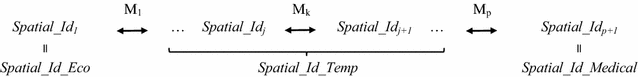
A mapping table for the IDs Spatial_Id_Medical and Spatial_Id_Eco IDs can be built by using p transition matrices (p ≥ 1). For example, a transition matrix makes it possible to associate each town’s spatial ID with the spatial ID of the state to which it belongs. However, in more complex situations, there may be no direct way of linking the two spatial IDs. Thus, two or more matrices are required, leading to the creation of at least one temporary spatial ID Spatial_Id_Temp. The mapping table yields p + 1 Spatial_Id, where Spatial_Id ₁ corresponds to the Spatial_Id_Eco and Spatial_Id _p+1 corresponds to the Spatial_Id_Medical. The transition matrices are based on a detailed assessment of the Spatial_Id_Medical and Spatial_Id_Eco IDs. It is then necessary to describe all the equivalence situations for each transition matrix. One or several Spatial_Id _j can correspond to one or several Spatial_Id _j+1 (1 ≤ j < p + 1). The various, mutually exclusive equivalence situations for a given transition matrix M_k (1 ≤ k ≤ p) are shown in Fig. 3.

Fig. 3

Mutually exclusive equivalence situations for a transition matrix M_k. M_k is a transition matrix from among M₁…M_p transition matrices. M_k describes the relationship between a Spatial_Id _j and a Spatial_Id _j+1 and therefore links them. n > 1, corresponds to the number of spatial IDs

Validation

Validation of the mapping table

After the final database has been built, it is necessary to validate the quality of the interface between the medical database and the ecological database. We used the following approach: (1) identification of the set of variables shared by the medical database and the ecological database; (2) choice of the variables that display the best exhaustiveness and reliability; and (3) comparison of these variables in the two databases on the scale of the SU_analysis spatial unit.

Spatial validation

In spatial terms, the final purpose of the mapping table is to create a background map on the scale of the SU_analysis spatial unit. In order to check the quality of the selected spatial unit (SU_analysis), it is necessary to evaluate spatial continuity and the decline in spatial resolution.

Spatial continuity is defined as the ability to move from any one point to another point without leaving the spatial unit considered. In other words, a spatially continuous unit has a single boundary [36,37,38]. A spatial unit that does not meet this condition is referred as discontinuous or fragmented. Most studies of putative links between a health outcome and environmental factors rely on the use of aggregated data. These data are frequently represented by the centroid of each spatial unit. However, in the case of discontinuous spatial units, the centroid may be outside the spatial unit. Hence, an error in the data’s spatial location (due to fragmented spatial units) might affect the findings and result in an erroneous conclusion [36,37,38]. In order to control for this eventuality, spatial continuity is evaluated by determining the fragmentation of the spatial units, defined as the number of discontinuous SU_analysis as a proportion of the total number of SU_analysis [37, 38]. This index can be calculated using geographical information systems, such as QGIS and ArcGIS [39, 40].

Spatial resolution is defined as the surface area of the smallest spatial unit in a given data set; it corresponds to the level of detail within the data. Aggregation of spatial units decreases the spatial resolution and thus the quality of the analysis. For example, the spatial resolution decreases if (for a given geographical zone) the data for a town are aggregated with data for the region as a whole. The decline in spatial resolution can initially be evaluated visually. The background map for SU_analysis is compared with the background map for the smallest spatial unit in the initial databases, in order to identify any obviously aberrant aggregates. The decline in spatial resolution can then be measured by calculating the ratio between the median surface area of SU_analysis and that of the smallest spatial unit in the initial databases (SU_initial = SU_eco or SU_med). This ratio must also be calculated for other administrative reference units whose surface area is known. These ratios are then compared: a lower index of decline corresponds to a spatial unit with a higher spatial resolution.

$$\frac{{{\text{SU\_analysis}}}}{{{\text{SU\_initial}}}}\quad {\text{versus}}\quad \frac{{{\text{SU\_reference1}}}}{{{\text{SU\_initial}}}}\quad {\text{versus}}\quad \frac{{{\text{SU\_reference2}}}}{{{\text{SU\_initial}}}}$$

For example, reference units 1 and 2 could be the county and the state for the USA, or the canton and the département for France. This index can be also calculated from census data on the number of inhabitants.

Application of the generic method: an illustrative example based on French databases

Data sources and objectives

In this section, the generic method is applied to a pair of French medical and ecological databases.

• 1. The medical database is the PMSI. Collection of these data has been approved by the French National Data Protection Commission (Commission Nationale de l’Informatique et des Libertés; authorization 1754053). The database is compiled and released by France’s Technical Agency for Information on Hospitalization (Agence Technique de l’Information sur l’Hospitalisation, ATIH). The database contains a summary of each inpatient stay in France, including the ICD-10 diagnostic code, the medical procedures performed (coded according to the French CCAM classification) and the patient’s age, gender, and unique identifier. Each patient is localized by his/her place of residence, which is only characterized by the PMSI spatial ID (Spatial_Id_PMSI) in the spatial unit SU_PMSI. There were 5644 distinct SU_PMSIs in France in 2014, which were characterized by a mean surface area of 97.37 km² and a mean population of 11,174.

• 2. The ecological database was produced by the INSEE [41]. The INSEE acts as France’s census office, and collects a vast range of demographic, social, economic and housing-related data. Most of the data are publicly available on the INSEE website. The data are summarized for various spatial units: the commune, the canton, the département and the région (in increasing hierarchical order; see Additional File 2 for details). Most frequently, the data are summarized on the scale of the commune (SU_INSEE), which is characterized by the spatial ID Spatial_Id_INSEE. In 2014, there were 36,594 communes (SU_INSEE) in France.

• 3. The spatial units SU_PMSI and SU_INSEE differ, as do the IDs Spatial_Id_PMSI and Spatial_Id_INSEE.

The goal of our method is to create a mapping table for the IDs Spatial_Id_PMSI and Spatial_Id_INSEE, in order to build a final database that includes both medical data from the PMSI and ecological data from the INSEE. The PMSI medical database provides information on each hospital stay for each patient, which are aggregated for each Spatial_Id_PMSI spatial unit. In this illustrative example, the healthcare event of interest is an in-hospital birth. This event was detected by screening for (1) hospital admissions from home, (2) a patient age of 7 days or less, (3) admissions from another hospital with a bodyweight below 2500 g, and (iv) admissions from another hospital, with a patient age below 30 days.

Construction rules

The direction of the relationship

The median [interquartile range (IQR)] surface area is larger for SU_PMSI (70 km² [21.6–147.6] than for SU_INSEE (10.8 km² [6.4–18.4]. Accordingly, the spatial unit for the analysis (SU_analysis) must be based on the spatial unit SU_PMSI, which is characterized by the spatial ID Spatial_Id_PMSI.

Transition matrices M₁, M₂

Two transition matrices were required to establish a correlation between Spatial_Id_INSEE and Spatial_Id_PMSI via the Zip_code:

The various equivalence situations for each transition matrix are presented in the Additional file 3. Transition matrix M1 is obtained by correlating Spatial_Id_INSEE (the ID for the communes) and the Zip_code for the commune [42]. In France, a zip code corresponds to the geographical zone covered by a single postal delivery office. The equivalence situations are described in detail in Table 1. In over 95% of cases, a given zip code covers several communes, which leads to the first data aggregation step (Table 1: situations 1, 4 and 5). In large, highly populated communes (< 1%), many zip codes correspond to a single commune. Each zip code corresponds to a single subset of the commune, and the union of these distinct subsets constitutes a commune (situation 2). In 5% of cases, the zip code corresponds to the commune’s Spatial_Id_INSEE (situation 3).

Table 1 Mapping table for Spatial_Id_INSEE and Spatial_Id_PMSI

Transition matrix M2 is obtained by correlating Spatial_Id_PMSI and Zip_code. According to the ATIH, Spatial_Id_PMSI has to be built from zip codes for legal reasons [43]. Thus, Spatial_Id_PMSI is equivalent to the zip code’s geographic area when the level of statistical confidentiality is high enough (in over 99% of cases; situations 1, 3 and 5). In the opposite case, Spatial_Id_PMSI corresponds to the aggregation of several zip codes (< 1% of cases: situations 2 and 4). A second aggregation step is then performed. In situation 2, the transition matrix M1 connects the commune to several zip codes. However, data partition is not necessary because the transition matrix M2 aggregates exactly the same units.

Lastly, a Spatial_Id_analysis ID is attributed to each of the Spatial_Id_PMSI (situations 1 to 4). The combination of transition matrix M1 and transition matrix M2 can, however, generate a small number of particular cases (< 1% of cases). In situation 5, several Spatial_Id_PMSI IDs have at least one Spatial_Id_INSEE ID in common. It is then impossible to obtain an exact correlation between the spatial ID from the PMSI and the spatial ID from the INSEE. In this situation, the Spatial_Id_PMSI IDs are aggregated into a single Spatial_Id_Analysis ID. Thus, 23 Spatial_Id_PMSI IDs were grouped into 11 Spatial_Id_Analysis IDs. In total, there were 5632 Spatial_Id_Analysis IDs in the final database.

The data processing and statistical analyses were performed using R software (version 3.3.2) [44]. QGIS software (version 2.14) was used to create the background map and calculate the fragmentation index [39].

Validation

Validation of the mapping table

In order to evaluate the quality of the match between the PMSI database and the INSEE database, the annual number of live births was used as the common variable.

The number of births associated with each Spatial_Id_INSEE ID was provided by the INSEE. The number of births associated with each Spatial_Id_PMSI ID was obtained by extracting the PMSI database.

For each Spatial_Id_Analysis ID, the indicators were compared by calculating the relative difference (i.e. the difference between the number of births in the INSEE data and the number of births in the PMSI data, divided by the number of births in the PMSI data). These relative differences are quoted as the median [IQR]. The total number of births was 785,742 in the INSEE database and 737,545 in the PMSI database, giving a difference of 48,197. The median [IQR] relative difference was 2.3% [0–5.7] (a boxplot is available in the Additional file 4).

In 2012, the ATIH performed an extensive study of the number of inhabitants in each SU_PMSI spatial unit, based on the INSEE data. The data on the number of inhabitants are available online for each Spatial_Id_PMSI [45]. We therefore transformed these data on the scale of the Spatial_Id_Analysis and compared the population data provided by the ATIH and the population data provided for SU_INSEE, as aggregated by our mapping table. For each of the Spatial_Id_Analysis IDs, the correlation was perfect (difference = 0). Hence, the resulting mapping table automatically performs the task described by the ATIH, regardless of the INSEE variable.

Spatial validation

A background map of the SU_analysis spatial unit was created using data from the French National Geographic Institute (Institut National de l’Information Géographique et Forestière, IGN) (Fig. 4). Spatial continuity was evaluated by calculating the fragmentation index; this was 2.4% (n = 134) for the 5632 SU_analysis spatial units. This value is within the range of fragmentation indices (2–40%) reported for public use microdata areas (PUMAs) in the USA [37].

Fig. 4

Background map for the SU_INSEE (a) and SU_analysis (b) in mainland France in 2014. a Background map of the spatial unit SU_INSEE, which represents the French communes in 2014. b Background map of the spatial unit SU_analysis, which represents the analysis spatial unit for our application in 2014

A possible decline in the spatial resolution was evaluated first by visual comparison of the respective background maps for SU_INSEE and SU_analysis (Fig. 4). The SU_analysis spatial unit appeared to be regularly distributed over the geographical zone, with no aberrant aggregations. In a second step, we calculated the decline index for the spatial resolution required to obtain data on the surface area and the number of inhabitants in the French communes, cantons and départements. The surface area data came from the IGN, whereas the data on the number of inhabitants came from the INSEE database. The comparison of the spatial resolution index for SU_analysis with the French administrative units is described in Table 2. The SU_analysis unit has a lower decline index than the cantons and départements for the surface area (6.5, 13.6 and 555.3, respectively) and the number of inhabitants (14.6, 24 and 1249.2, respectively).

Table 2 Comparison of the numbers of inhabitants and surface areas

On average, the spatial unit for analysis is therefore 6 times larger than the smallest available unit, testifying to a loss of spatial resolution. However, our method minimizes this loss; for the surface area, the scale is twice as fine as the first reference unit (the canton) and nearly 100 times finer than for the département (the second reference unit).

As an illustrative example of the application of this method, the birth rate was mapped (Additional file 5).

Discussion

The method presented here addresses the interoperability problem for ecological and medical databases in a context of the spatial analysis of healthcare events. The loss of spatial resolution was minimized, and we did not have to resort to the use of spatial disaggregation techniques. The method’s application to French national data enabled us to correlate medical data from the PMSI database with ecological data from the INSEE database—resulting in the creation of a final database for fine-scale spatial analysis.

This method may be of value for correlating ecological and medical big data in spatial analyses. This type of data is increasingly available and is opening up new perspectives in epidemiology. However, the use of medical big data in the field of spatial analysis is restrained by interoperability problems, known as the change-of-support problem and the misaligned data problem [26]. In Rossheim et al.’s study of alcohol sales and the socio-economic environment, the data were available on the scale of the zip code, the census block or the zip code tabulation area. To perform analyses on the zip code scale, the researchers were obliged to use spatial disaggregation and aggregation methods; this decreased the quality of the final spatial analysis database [46]. A similar problem was encountered in Sundmacher and Busse’s study of the link between physician supply and avoidable cancer deaths in Germany. The lack of interoperability and the broad range of ecological databases prompted the researchers to use spatial interpolation methods on the district level and to not integrate certain environmental data—thus placing limitations on their analyses [47].

Spatial resolution is a major issue in the spatial analysis of healthcare data because it is easier to detect local phenomena when the resolution is high [30]. For example, the decrease in spatial resolution affects the precision with which a cluster can be localized [8, 48]. The variation in the results of a spatial analysis as a function of the spatial resolution was emphasized by Lee et al.’s study of obesity in the USA; fewer healthcare events were identified when the spatial resolution fell [49]. Jeffery et al. [50] came to a similar conclusion in their study of paediatric leukemia.

The advantage of our method consists in opting for aggregation on the finest scale possible, whilst checking the quality of the final spatial analysis database. This approach appears to have been used previously in a study of stroke, although the method’s details were not specified [23]. The use of spatial disaggregation methods is not desirable, since they lead to a loss of precision in spatial analysis—even when complex models are used [26, 34]. Furthermore, validation of the mapping table results in a high-quality final database for spatial analysis. The spatial validation process ensures that the greatest possible spatial resolution is achieved. Lastly, validation ensured that the spatial units’ fragmentation index remains low. By way of an example, Siordia et al.’s studies of the American PUMA database featured a high fragmentation index and thus encountered theoretical difficulties in the application of statistical models; the spatial position of a healthcare event was no longer coherent with that of a spatial unit [37, 38]. This generic method may provide a structural framework so that researchers can provide a standardized description of the methods used to aggregate ecological and medical spatial data.

Nevertheless, our present method has a number of limitations, most of which are inherent to all spatial analyses. Firstly, a large percentage of the scenario 5 (Table 1) might decrease the spatial resolution, due to the aggregation of several basic spatial units. This issue can be evaluated by analyzing the spatial resolution index (as presented in the present study) and establishing whether the final spatial unit sizes are homogeneously distributed or not. Secondly, the geographical boundaries of spatial units change over time, which can make it more difficult to study healthcare events over a long time interval. This problem can be tackled in two ways: by optimizing the study period and thus minimizing changes in geographical boundaries or by considering the geographic boundaries that correspond to the longest study period. Thirdly, our method only partly addressed the change-of-support problem because it only applies to aggregated data (a frequent situation in the spatial analysis of healthcare events, nevertheless) [51]. Therefore, for other types of spatial data (such as geostatistical data), preliminary work on aggregation to the spatial unit of interest must be carried out in collaboration with specialists in the particular field. Lastly, the present method requires the definition of transition matrices prior to construction of the mapping table.

Conclusion

In conclusion, the present work suggests that it is possible to significantly improve the interoperability of ecological databases and medical databases, and thus enable finer-scale analyses. In view of the growing availability of big data, the method presented here could be a useful tool for the precise spatial analysis of large geographical areas.

References

Tatem AJ, Jia P, Ordanovich D, Falkner M, Huang Z, Howes R, et al. The geography of imported malaria to non-endemic countries: a meta-analysis of nationally reported statistics. Lancet Infect Dis. 2017;17:98–107.
Burke M, Heft-Neal S, Bendavid E. Sources of variation in under-5 mortality across sub-Saharan Africa: a spatial analysis. Lancet Glob Health. 2016;4:e936–45.
Duncan EW, White NM, Mengersen K. Bayesian spatiotemporal modelling for identifying unusual and unstable trends in mammography utilisation. BMJ Open. 2016;6:e010253.
Vine MF, Degnan D, Hanchette C. Geographic information systems: their use in environmental epidemiologic research. Environ Health Perspect. 1997;105:598–605.
Takahashi K, Tachimori H, Kan C, Nishi D, Okumura Y, Kato N, et al. Spatial analysis for regional behavior of patients with mental disorders in Japan. Psychiatry Clin Neurosci. 2017;71:254–61.
Gower-Rousseau C. Epidémiologie des maladies inflammatoires chroniques de l’Intestin en France : apport du registre EPIMAD. phdthesis. Université du Droit et de la Santé—Lille II; 2012. https://tel.archives-ouvertes.fr/tel-00820631/document. Accessed 20 Dec 2016.
Declercq C, Gower-Rousseau C, Vernier-Massouille G, Salleron J, Baldé M, Poirier G, et al. Mapping of inflammatory bowel disease in northern France: spatial variations and relation to affluence. Inflamm Bowel Dis. 2010;16:807–12.
Jones SG, Kulldorff M. Influence of spatial resolution on space-time disease cluster detection. PloS One. 2012;7:e48036.
Kulldorff M, Nagarwalla N. Spatial disease clusters: detection and inference. Stat Med. 1995;14:799–810.
Besag J, York J, Mollié A. Bayesian image restoration, with two applications in spatial statistics. Ann Inst Stat Math. 1991;43:1–20.
Bambhroliya AB, Burau KD, Sexton K. Spatial analysis of county-level breast cancer mortality in Texas. J Environ Public Health. 2012;2012:959343.
Meliker JR, Jacquez GM, Goovaerts P, Copeland G, Yassine M. Spatial cluster analysis of early stage breast cancer: a method for public health practice using cancer registry data. Cancer Causes Control CCC. 2009;20:1061–9.
Sánchez-Díaz G, Arias-Merino G, Villaverde-Hueso A, Morales-Piga A, Abaitua-Borda I, Hens M, et al. Monitoring Huntington’s disease mortality across a 30-year period: geographic and temporal patterns. Neuroepidemiology. 2016;47:155–63.
Goungounga JA, Gaudart J, Colonna M, Giorgi R. Impact of socioeconomic inequalities on geographic disparities in cancer incidence: comparison of methods for spatial disease mapping. BMC Med Res Methodol. 2016;16:136.
Toga AW, Foster I, Kesselman C, Madduri R, Chard K, Deutsch EW, et al. Big biomedical data as the key resource for discovery science. J Am Med Inform Assoc JAMIA. 2015;22:1126–31.
Yildirim O, Gottwald M, Schüler P, Michel MC. Opportunities and challenges for drug development: public-private partnerships, adaptive designs and big data. Front Pharmacol. 2016;7:461.
Barrett MA, Humblet O, Hiatt RA, Adler NE. Big data and disease prevention: from quantified self to quantified communities. Big Data. 2013;1:168–75.
Sparks R, Lau WW, Tsang JS. Expanding the immunology toolbox: embracing public-data reuse and crowdsourcing. Immunity. 2016;45:1191–204.
Marco-Ruiz L, Moner D, Maldonado JA, Kolstrup N, Bellika JG. Archetype-based data warehouse environment to enable the reuse of electronic health record data. Int J Med Inf. 2015;84:702–14.
Fletcher-Lartey SM, Caprarelli G. Application of GIS technology in public health: successes and challenges. Parasitology. 2016;143:401–15.
Ribeiro AI, Olhero A, Teixeira H, Magalhães A, Pina MF. Tools for address georeferencing—limitations and opportunities every public health professional should be aware of. PloS One. 2014;9:e114130.
Beuscart J-B, Genin M, Dupont C, Verloop D, Duhamel A, Defebvre M-M, et al. Potentially inappropriate medication prescribing is associated with socioeconomic factors: a spatial analysis in the French Nord-Pas-de-Calais Region. Age Ageing. 2017;46(4):607–613.
Roussot A, Cottenet J, Gadreau M, Giroud M, Béjot Y, Quantin C. The use of national administrative data to describe the spatial distribution of in-hospital mortality following stroke in France, 2008–2011. Int J Health Geogr. 2016;15:2.
A. Kadadi, R. Agrawal, C. Nyamful, R. Atiq. Challenges of data integration and interoperability in big data. In: 2014 IEEE international conference on big data (big data). 2014. p. 38–40.
Devogele T, Parent C, Spaccapietra S. On spatial database integration. Int J Geogr Inf Sci. 1998;12:335–52.
Gotway CA, Young LJ. Combining incompatible spatial data. J Am Stat Assoc. 2002;97:632–48.
Evain F. À quelle distance de chez soi se fait-on hospitaliser ? Etudes Résultats Drees. 2011. http://drees.social-sante.gouv.fr/IMG/pdf/er754-2.pdf. Accessed 15 Dec 2016.
Le Bail M, Or Z. Atlas des variations de pratiques médicales. Recours à dix interventions chirurgicales. 2016. www.irdes.fr/recherche/ouvrages/002-atlas-des-variations-de-pratiques-medicales-recours-a-dix-interventions-chirurgicales.pdf.
Canto MT, Anderson WF, Brawley O. Geographic variation in breast cancer mortality for white and black women: 1986–1995. CA Cancer J Clin. 2001;51:367–70.
Beale L, Abellan JJ, Hodgson S, Jarup L. Methodologic issues and approaches to spatial epidemiology. Environ Health Perspect. 2008;116:1105–10.
Elliott P, Wartenberg D. Spatial epidemiology: current approaches and future challenges. Environ Health Perspect. 2004;112:998–1006.
Bureau of Health Informatics Office of Quality and Patient Safety. SPARCS Operations Guide. 2016. https://www.health.ny.gov/statistics/sparcs/training/docs/sparcs_operations_guide.pdf. Accessed 16 Dec 2016.
Health and social care information centre. HES Data Dictionary: Admitted Patient Care. 2017. http://content.digital.nhs.uk/media/23711/Admitted-Patient-Care/pdf/Admitted_Patient_Care_.pdf. Accessed 10 Mar 2017.
Li T, Pullar DV, Corcoran J, Stimson RJ. A comparison of spatial disaggregation techniques as applied to population estimation for south east Queensland (SEQ), Australia. Appl GIS. 2007;3:1–16.
Spatial Disaggregation & Small-Area Estimation Methods for Agri. Surveys: Solutions & Perspectives. 2015. http://gsars.org/wp-content/uploads/2015/09/TR-Spatial-Disaggregation-and-Small-Area-Estimation-210915.pdf.
Grubesic TH, Matisziw TC. On the use of ZIP codes and ZIP code tabulation areas (ZCTAs) for the spatial analysis of epidemiological data. Int J Health Geogr. 2006;5:58.
Siordia C, Wunneburger DF. Contiguity principle for geographic units: evidence on the quantity, degree, and location of Public Use Microdata Area (PUMA) fragmentation. Hum Geogr—J Stud Res Hum Geogr. 2013;7:5–13.
Siordia C, Fox A. Public use microdata area fragmentation: research and policy implications of polygon discontiguity. Spat Demogr. 2013;1:41–55.
QGIS Development Team. QGIS Geographic Information System. 2009.
Environmental Systems Research Institute. ArcGIS. 2011.
Institut national de la statistique et des études économiques. https://www.insee.fr.
Open data soft. Correspondance Code INSEE—Code Postal 2013. https://public.opendatasoft.com/explore/dataset/correspondance-code-insee-code-postal/. Accessed 15 Dec 2016.
Atih. Mise à jour 2014 de la liste de correspondance codes postaux codes géographiques. 2015. http://www.atih.sante.fr/mise-jour-2014-de-la-liste-de-correspondance-codes-postaux-codes-geographiques. Accessed 16 Dec 2016.
R Core Team. R: a language and environment for statistical computing. Vienna: R Foundation for Statistical Computing; 2016. https://www.R-project.org/.
Atih. Mise à jour 2015 de la liste de correspondance codes postaux codes géographiques PMSI. 2015. http://www.atih.sante.fr/mise-jour-2015-de-la-liste-de-correspondance-codes-postaux-codes-geographiques. Accessed 16 Dec 2016.
Rossheim ME, Thombs DL, Wagenaar AC, Xuan Z, Aryal S. High alcohol concentration products associated with poverty and state alcohol policies. Am J Public Health. 2015;105:1886–92.
Sundmacher L, Busse R. The impact of physician supply on avoidable cancer deaths in Germany. A spatial analysis. Health Policy Amst Neth. 2011;103:53–62.
Olson KL, Grannis SJ, Mandl KD. Privacy protection versus cluster detection in spatial epidemiology. Am J Public Health. 2006;96:2002–8.
Lee J, Alnasrallah M, Wong D, Beaird H, Logue E. Impacts of scale on geographic analysis of health data: an example of obesity prevalence. ISPRS Int J Geo-Inf. 2014;3:1198–210.
Jeffery C, Ozonoff A, Pagano M. The effect of spatial aggregation on performance when mapping a risk of disease. Int J Health Geogr. 2014;13:9.
Gelfand AE, Zhu L, Carlin BP. On the change of support problem for spatio-temporal data. Biostat Oxf Engl. 2001;2:31–45.
Authors’ contributions
AG and MG developed the method and performed analyses. All authors were major contributors in writing the manuscript. All authors read and approved the final manuscript.
Acknowledgements
David Fraser who provided professional writing services.
Competing interests
The authors declare that they have no competing interests.
Availability of data and material
The datasets analysed during the current study are available on the Open data soft website [42], the Atih website [43, 45] and the INSEE website [41].
Consent for publication
All authors agree to the terms of the BioMed Central Copyright and License Agreement.
Ethics approval and consent to participate
Collection of medical data has been approved by the French National Data Protection Commission (Commission Nationale de l’Informatique et des Libertés; authorization 1754053).
Publisher’s Note
Springer Nature remains neutral with regard to jurisdictional claims in published maps and institutional affiliations.
Author information
Authors and Affiliations
Corresponding author
Additional files
12942_2017_109_MOESM2_ESM.pdf
Additional file 2. Description of the French administrative spatial units in terms of frequencies, surface area (in km2) and number of inhabitants. The different circles indicate the hierarchical relationships between the different administrative units.
12942_2017_109_MOESM3_ESM.pdf
Additional file 3. Equivalence situations for the transition matrices M1 and M2. Matrix 1 is the tool used to link the Spatial_Id_INSEE and the Zip_Code. Matrix 2 is the tool used to link the Zip_Code and the Spatial_Id_PMSI. “Yes” indicates situations encountered in the application.
12942_2017_109_MOESM4_ESM.pdf
Additional file 4. Relative difference in the number of births per spatial unit SU_analysis between the ecological data from the INSEE and the medical data from the PMSI.
12942_2017_109_MOESM5_ESM.png
Additional file 5. Birth rate for 10,000 inhabitants for the SU_INSEE (A) and SU_analysis (B). The first map (A) is on the scale of the commune spatial unit (SU_INSEE), and represents the birth rate calculated from the number of births and the underlying population data in the INSEE database. The second map (B) is on the scale of the SU_analysis spatial unit, and represents the birth rate per 10,000 inhabitants calculated using the number of births in the PMSI database and the underlying population data in the INSEE database.
Rights and permissions
Open Access This article is distributed under the terms of the Creative Commons Attribution 4.0 International License (http://creativecommons.org/licenses/by/4.0/), which permits unrestricted use, distribution, and reproduction in any medium, provided you give appropriate credit to the original author(s) and the source, provide a link to the Creative Commons license, and indicate if changes were made. The Creative Commons Public Domain Dedication waiver (http://creativecommons.org/publicdomain/zero/1.0/) applies to the data made available in this article, unless otherwise stated.
About this article
Cite this article
Ghenassia, A., Beuscart, J.B., Ficheur, G. et al. A generic method for improving the spatial interoperability of medical and ecological databases. Int J Health Geogr 16, 36 (2017). https://doi.org/10.1186/s12942-017-0109-5
Received:
Accepted:
Published:
DOI: https://doi.org/10.1186/s12942-017-0109-5